MS EXCEL solution

1.EXAMPLE SOLUTION

2.EXAMPLE SOLUTION

3.EXAMPLE SOLUTION

4.EXAMPLE SOLUTION

5.EXAMPLE SOLUTION

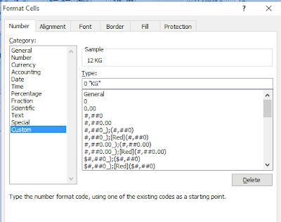
REMOVE KG IN QUANTITY USING FIND AND RAPLACE
PRESS CTRL+1

6.EXAMPLE SOLUTION

CREATE CUSTOM LIST
SELECT DATE OR MONTH CELLS
PRESS ALT+A+S
SORT BY MONTH IN ORDER BY CUSTOM LIST

7.EXAMPLE SOLUTION

8.EXAMPLE SOLUTION

9.EXAMPLE SOLUTION

SELECT ANY CELL

PRESS ALT+N+V

DOWNLOAD PIVOT TABLE FILE

10.NEED TO IDENTIFY HOW MANY STUDENT

PRESENT AND ABSENT USING FORMULA

11.EXAMPLE SOLUTION

12.EXAMPLE SOLUTION

13.EXAMPLE SOLUTION

14.EXAMPLE SOLUTION

15.EXAMPLE SOLUTION

How to create this dynamic heat map?

Here is the complete data set that is used to create this dynamic heat map.

Here are the steps:

In a new sheet (or in the same sheet), enter the month names (simply copy paste it from the original data).
Go to Developer –> Controls –> Insert –> Scroll Bar. Now click anywhere in the worksheet, and it will insert a scroll bar.

Right-click on the scroll bar and click on Format Control.

In the Format Control dialog box, make the following changes:

Minimum Value: 1
Maximum Value 5
Cell Link: Sheet1!$J$1 (You can click on the icon in the right and then manually select the cell you want to link to the scroll bar).

Click OK.
In cell B1, enter the formula: =INDEX(Sheet1!$B$1:$H$13,ROW(),Sheet1!$J$1+COLUMNS(Sheet2!$B$1:B1)-1)
Resize and place the scroll bar at the bottom of the data set.

Now when you change the scroll bar, the value in Sheet1!$J$1 would change, and since the formulas are linked to this cell, it would update to show the correct values.